Division in Hardware

The pre-requisite for this post includes the knowledge of basic boolean algebra, solid background on Digital Electronics is a big plus. Majority of the content on the internet talks about the sequential architecture of the division algorithm. However, irrespective of the same idealogy it is difficult to visualise the combinatorial division circuit. The posts on combination multiplier are readily available on the internet one such post is Multiplier Architecture .

In this post, I will try to cover the concept behind the restoring and the non-restoring type division algorithms and then translate these algorithms to respective hardware architecture.

Let’s start with the school book division. The four generic terms used in every division algorithm are dividend, divisor, quotient and remainder. The following image shows the naive division algorithm and an equivalent which will be used to build the understanding.

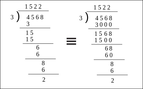
Fig:Naive division method.

In the figure Dividend=4568, Divisor(D)=3, Quotient(q)=1522 and Remainder(R)=2. Now, the division takes four steps, the \(i^{th}\) digit of q is denoted as \(q_{i}\) and the partial remainder at the \(i^{th}\) step after substraction is denoted as R(i). Assume that R(0) is the final remainder. Looking at the division once again we observe.

\(4568 - 1*3*10^{3}=1568\) or R(4) - \(q_{3}*D*10^{3}\)= R(3)

\(1568 - 5*3*10^{2}=0068\) or R(3) - \(q_{2}*D*10^{2}\)= R(2)

\(0068 - 2*3*10^{1}=0008\) or R(2) - \(q_{1}*D*10^{1}\)= R(1)

\(0008 - 1*3*10^{0}=0002\) or R(1) - \(q_{0}*D*10^{0}\)= R(0)

R(4) is numerically equal to the dividend. Now, observing the sequence we can say that the Remainder, in general, can be expressed as:

where \(i= n-1, n-2, ......, 1, 0\).

Now, the whole purpose of introducing the naive approach is the fact that in binary-only the radix changes from 10 to 2. The inherent concept remains the same, one important questions to ask at this point is how the quotient \(q_{i}\) is calculated? It is obvious that through observation we figure out the value of quotient at every iteration but for a machine, we need to define a methodology as an alternative to this observation. Further, this observation is nothing but a mental trial and error. We keep on checking the difference between the partial remainder (dividend in the first step) and the integer multiple of the divisor till the point we get a negative value. Once the integer multiple yielding the negative difference is obtained we choose the \(q_{i}\) as one less than that particular integer. This is the main idea of restoring division.

Restoring Divison

As discussed in the previous paragraph the restoring division also gives a positive partial remainder. The examples from here onwards will deal with radix as 2 instead of 10 as discussed in the previous paragraphs. In case of 2 as the radix, the quotient is either 0 or 1 so using \eqref{division_gen} and rewriting the equation.

We start with assuming \(q_{i}\) as 1 so

Now from here onwards we define two cases based on the value of \(R(i)\).

Case 1: if \(R(i) \geq 0\) the assumption for \(q_{i}\)=1 was correct.

Case 2: if \(R(i) < 0\) the assumption was wrong and we need to restore the partial remainder.

Let’s understand this with an example.

\(29 - 3*2^{4} = -19 \ \ q_{4}=1\) (R(4) < 0 : restore)

\(-19 + 3*2^{4}= +29 \ \ q_{4}=0\) (R(4) \(\geq\) 0 : continue)

\(29 - 3*2^{3}= +5 \ \ q_{3}=1\) (R(3) \(\geq\) 0: continue)

\(+5 - 3*2^{2}= -7 \ \ q_{2}=1\) (R(2) < 0 : restore)

\(-7 + 3*2^{2}= +5 \ \ q_{2}=0\) (R(2) \(\geq\) 0 : continue)

\(+5 - 3*2^{1}= -1 \ \ q_{1}=1\) (R(1) < 0 : restore)

\(-1 + 3*2^{1}= +5 \ \ q_{1}=0\) (R(1) \(\geq\) 0: continue)

\(+5 - 3*2^{0}=+2 \ \ q_{0}=1\) (R(0) \(\geq\) 0 : continue)

Now using the \(q_{i}\) values where continue keyword is used the quotient obtained is 01001 which is equivalent to 9 which should be the actual quotient. Let’s look into another example with boolean values.

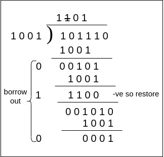
Fig: Binary Restoring Division with Dividend=46, Divisor=9, Quotient=5, Remainder= 1.

Now looking at the example it is trivial that we need to have a subtractor in our design. Moreover, to mitigate the extra step present to restore the partial remainder we can think of an architecture which directs the partial remainder to the next iteration upon checking whether the result of subtraction is negative. To sum up we will use a multiplexer with final borrow out as the selection line which is 1 if the subtraction is negative and 0 when it is positive. To understand the binary full subtractor refer to this post Binary Subtractor. One important point to note is the binary division considered here is for unsigned binary numbers with the divisor and dividend aligned. As mentioned earlier our main aim is to design a combinatorial divisor, so it is evident that we need an array-like structure to incorporate the bitwise operations. Let’s discuss the building block of this array structure.

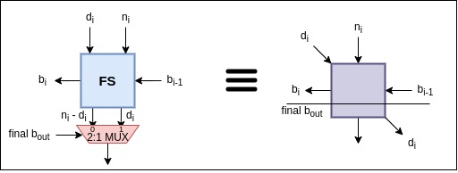
Fig: Array architecture building block Restoring Divider.

The \(final\ b_{out}\) is calculated from the block present at the Main Significant Bit (MSB). Furthermore, it is important to realise that the architecture proposed can be extended to floating-point by continuing the iterations for the sake of simplicity we only consider the integer quotient. Now with the help of the building blocks, we can construct an array architecture for restoring division which is purely combinatorial. Here for the architecture we have considered the dividend as 6 bits (\(n_5 n_4 n_3 n_2 n_1 n_0\)), the divisor is 4 bits (\(d_3 d_2 d_1 d_0\)), the quotient is 3 bits (\(q_2 q_1 q_0\)) Why? To answer this first understand the assumption that the dividend and the divisor are aligned which means the MSB’s of both the binary representation has 1 as its value. So, maximum quotient can be calculated as \(\frac{max\ dividend}{min\ divisor}\) which comes out to be \(\frac{63}{8}\) taking the \(log_2\) followed by the ceiling of the value we obtain 3. How about you check it out yourself?. Finally, the remainder is expressed as 4 bits (\(r_3 r_2 r_2 r_0\)).

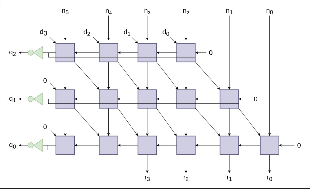
Fig: Array architecture Restoring Divider.

The quotient bit as seen from the figure is the inverted form of the \(final\ b_{out}\). Also, the initial borrow input is given as 0 which is trivial. The number of rows in the array architecture is given as \(rows = width\ of \ dividend\ - \ width\ of \ divisor\ + \ 1\). The number of rows corresponds directly to the width of the quotient, which can be proved intuitively using the stated assumption and the example calculation in the previous paragraph. Moreover, if the divisor and the dividend are aligned perfectly we can remove the first block in the third row from the left.

Non-restoring Division

The idea of restoring division can be extended using simple manipulation such that the restoration of the partial remainder is omitted. To understand this manipulation let’s look at it mathematically.

From the previous equation we know.

\(R(i)= R(i+1) - D*2^{i}\\\) Case 1: We need to restore when R(i) < 0 this is done by adding \(D*2^{i}\)

\(R(i)= R(i) + D*2^{i} \\\) Now, in the next iteration we subtract \(D*2^{i-1}\) for the assumption \(q_{i}=1\)

\(R(i-1)= R(i) - D*2^{i-1} \\\) \(R(i-1)=R(i) + D*2^{i} - D *2^{i-1}\\\) \(R(i-1)=R(i) + D*2^{i-1} \\\) Case 2: When \(R(i) \geq 0\) the assumption was correct for \(q_{i}=1\) continue.

The Non-restoring division algorithm doesn’t need to restore the partial remainder every time rather if the partial remainder is negative we need to add the divisor in the next iteration taking into consideration the bit shifts. To obtain this functionality with minimal hardware we need to look at the combined hardware used for addition and subtraction of binary bits. Refer to the section Binary Adder Subtractor in the post Binary Subtractor . The combined hardware used works on the principle that the subtraction can be performed using the 2’s complement notation. According to this method first, the binary number to be subtracted is converted in 2’s complement notation by inverting its bits and adding 1 to it. Further, the 2’s complemented number is then added to another operand. Refer to this post to gain insight on the 2’s complement subtraction Subtraction by 2’s complement . Finally, the most important point to address here is the fact that when subtraction is done using the adder hardware with one input complemented and initial carry input as 1, the output is considered negative if the final carry out is 0 and positive when the final carry out is 1. This concept will be used extensively in the later sections.

\(29 - 3*2^{4} = -19 \ \ q_{4}=1\) (R(4) < 0: assumption wrong)

\(-19 + 3*2^{3}= +5 \ \ q_{3}=\bar{1}\) (R(3) \(\geq\) 0: continue)

\(+5 - 3*2^{2}= -7 \ \ q_{2}=1\) (R(2) < 0: assumption wrong)

\(-7 + 3*2^{1}= -1 \ \ q_{2}=\bar{1}\) (R(1) < 0: assumption wrong)

\(-1 + 3*2^{0}= 2 \ \ q_{1}=\bar{1}\) ( R(0) \(\geq\) 0: continue post decimal)

From the example we observe that non restoring algorithm takes lesser number of iterations compared to the restoring algorithm. However as you can observe the quotient bits are not in the form of normal 0 and 1 rather in the form of 1 and \(\bar{1}\) which has a numerial value equivalent to -1. So here the quotient obtained is \(1 \bar{1} 1 \bar{1} \bar{1}\) numrically calculated as \(1*2^{4} -1*2^{3} + 1*2^{2} - 2*2^{1} -1*2^{0} = 9\).

Now, let’s look at another example of non-restoring division algorithm with boolean values. In the example, we will perform subtraction using the 2’s complement notation used in the combined adder subtractor circuit mentioned previously. Thus, the subtraction results with final carry out as 0 has a negative value and the subtraction with carry out as 1 has a positive value.

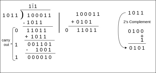
Fig: Binary Non-restoring Division with Dividend=35, Divisor=11, Quotient=3, Remainder=2.

Considering the example and the discussion in the previous paragraph it is easy to guess that we need a combined adder subtracter circuit which performs addition if the carry out from the previous iteration is 0 (a negative value) and performs the normal subtraction of the carry out from the previous iteration is 1 ( a positive value).

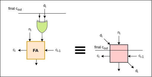
Fig: Array architecture building block Non restoring divider.

The \(final\ c_{out}\) is obtained through the block present at the MSB. Again, if the requirement of quotient bit is higher one can extend the architecture. Now, let’s construct the array architecture for the Non-restoring array divider with the dividend as 6 bits (\(n_5 n_4 n_3 n_2 n_1 n_0\)), the divisor as 4 bits (\(d_3 d_2 d_1 d_0\)), the quotient as 3 bits (\(q_2 q_1 q_0\)) and the remainder as 4 bits (\(r_3 r_2 r_1 r_0\)).

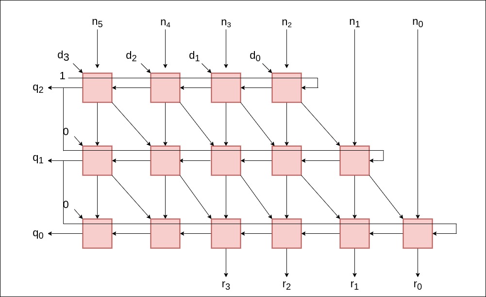
Fig: Array architecture Non restoring Divider.

Looking at the array structure we need to address the two main points. First, in the topmost row, the value of the \(final \ c_{out}\) is 1, this is because the first iteration is always subtraction in the non-restoring divider. Second, as observed above in the example of binary Non restoring divider the quotient bits are not of form 0 or 1 rather it is of form 1 and \(\bar{1}\). The conversion of to the original encoding scheme can be done after storing the 0,1 sequence of the quotient bit depending on the order since we know the first is always 1 and then if 0 appears means the next quotient bit is \(\bar{1}\). Moreover, if the input and the outputs are perfectly aligned then the first block in the third row from the left can be completely omitted.

Interested readers can visit the Lecture Notes of EE486 Advanced Computer Arithmetic by Prof. M.J.Flynn Stanford University. Furthermore, I am thankful to Prof. A.S.Dhar for the course on Architectural Design of Integrated Circuits at IIT Kharagpur.